Smooth a tide record

Download the tide data. In this case 2 days of tides at the Cascais tide gauge station.

using GMT

D = maregrams(code="casc", starttime="2025-03-05T13:26:00")

Attribute table
┌─────────┬─────────┬──────────┬─────────┐
│ ST_name │ ST_code │  Country │ Timecol │
├─────────┼─────────┼──────────┼─────────┤
│ Cascais │    casc │ Portugal │       1 │
└─────────┴─────────┴──────────┴─────────┘
BoundingBox: [1.74118116e9, 1.74135396e9, -0.679, 1.441]

30189×2 GMTdataset{Float64, 2}
 Row │                time  rad(m) 
─────┼─────────────────────────────
   1 │ 2025-03-05T13:26:00  -0.508
   2 │ 2025-03-05T13:26:05  -0.519
   3 │ 2025-03-05T13:26:10  -0.507
   4 │ 2025-03-05T13:26:15  -0.502
   5 │ 2025-03-05T13:26:20  -0.517
   6 │ 2025-03-05T13:26:25  -0.529
   7 │ 2025-03-05T13:26:30  -0.501
   8 │ 2025-03-05T13:26:35  -0.515
  ⋮  │          ⋮             ⋮

using GMT

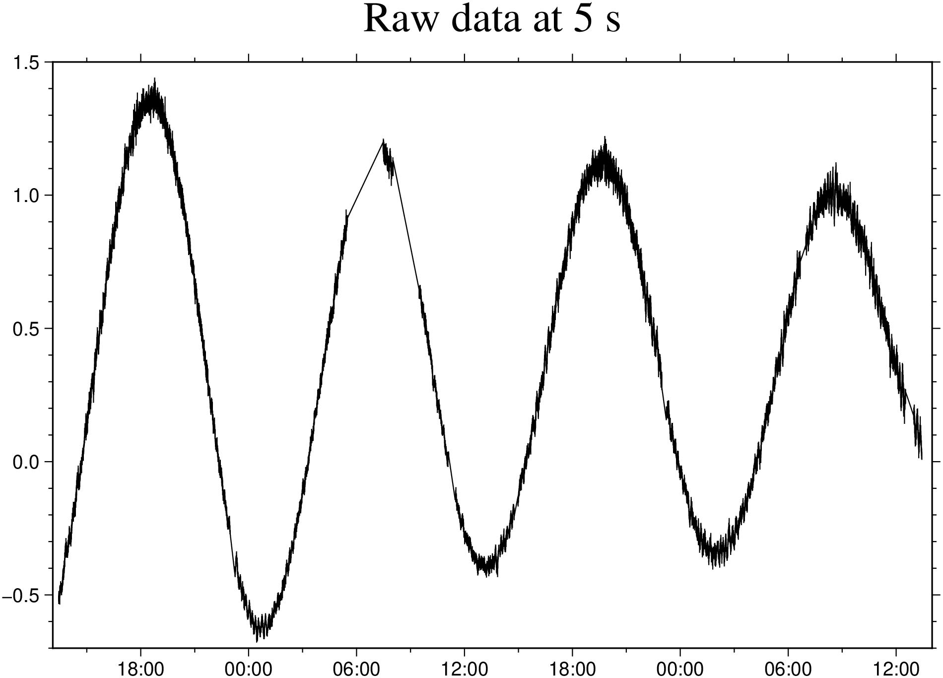
viz(D, title="Raw data at 5 s")

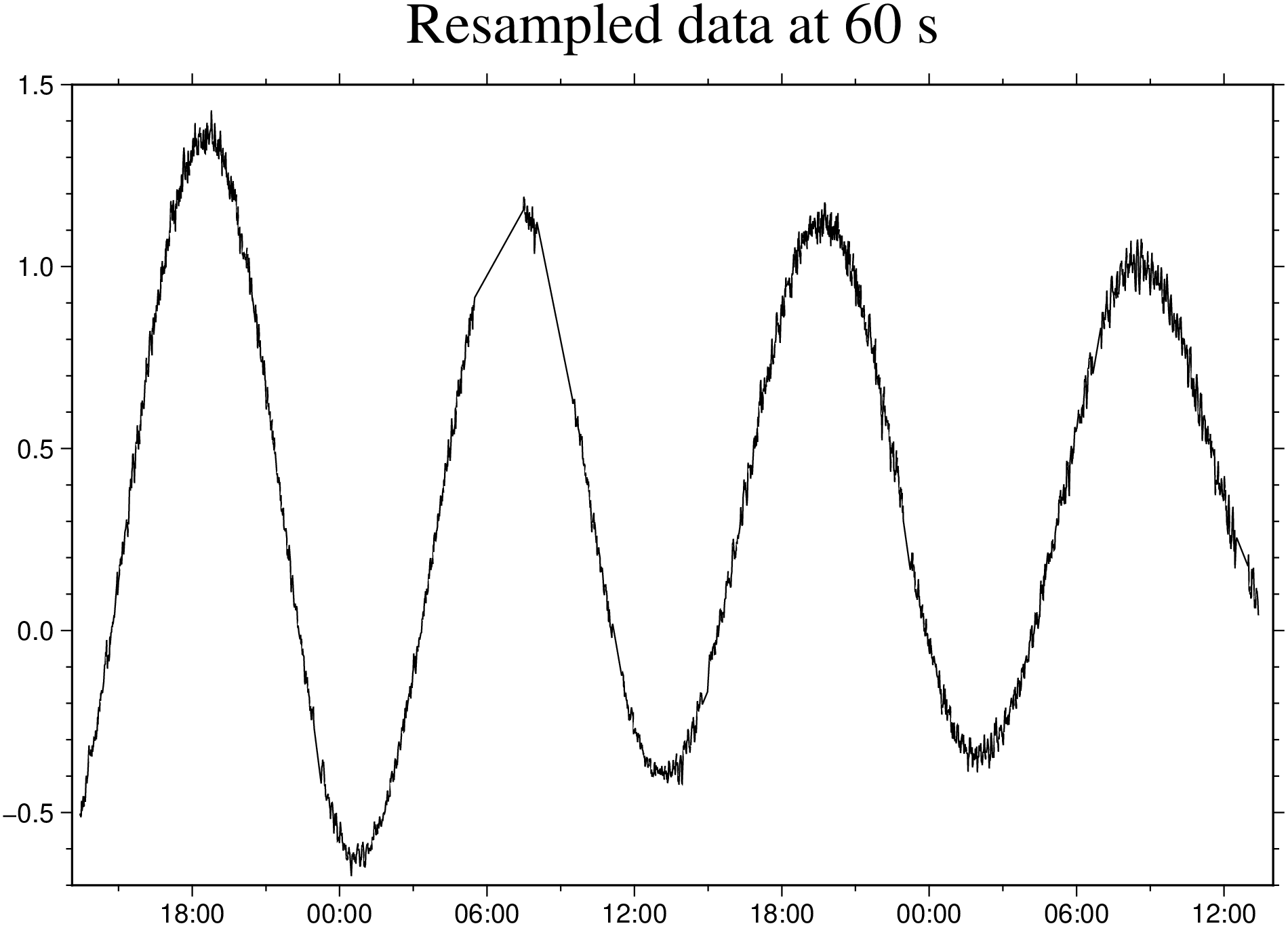
Resample data to 60 seconds intervals and break at gaps > 300 s. The nonans option is used to remove rows with NaN values that otherwise would be present inside the gaps.

Ds = sample1d(D, T="2025-03-05T13:26:00/2025-03-07T13:24:05/60s", g="x300s", nonans=1);

# The above Dataset is made up of 9 segments. _size(Ds)_ shows just that.
size(Ds)

(9,)

Let's stack them up to get a single segment using the stack function.

A plot of the data is similar to that of the raw data, but with much less points (points every 60 s instead of every 5 s).

Dt = stack(Ds);
viz(Dt, title="Resampled data at 60 s")

Now we are going to do the first step of the filtering process using the lowess function. This function fits a non-parametric regression model to the data using locally weighted linear regression. The span parameter is a factor that controls the smoothing and delta helps speeding up the calculus but experience have show that it also affects curvature of the obtained curve. Note: obtaining the values for these parameters is a trial and error process.

Dl = lowess(Dt, span=0.02, delta=200);
viz(Dl, title="Lowess smoothed data at 60 s")

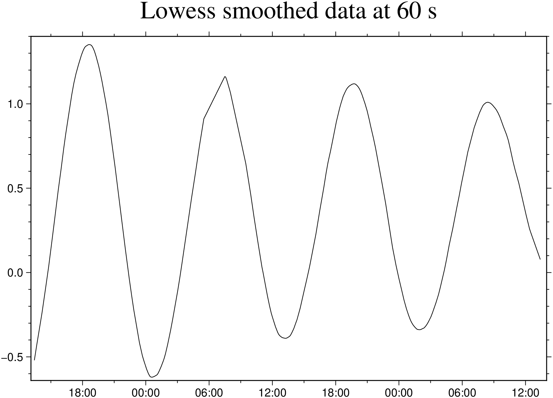
Much nicer and we almost there but not yet because we can see that the curve still has the gaps. To fill them we are going to use the sample1d function again.

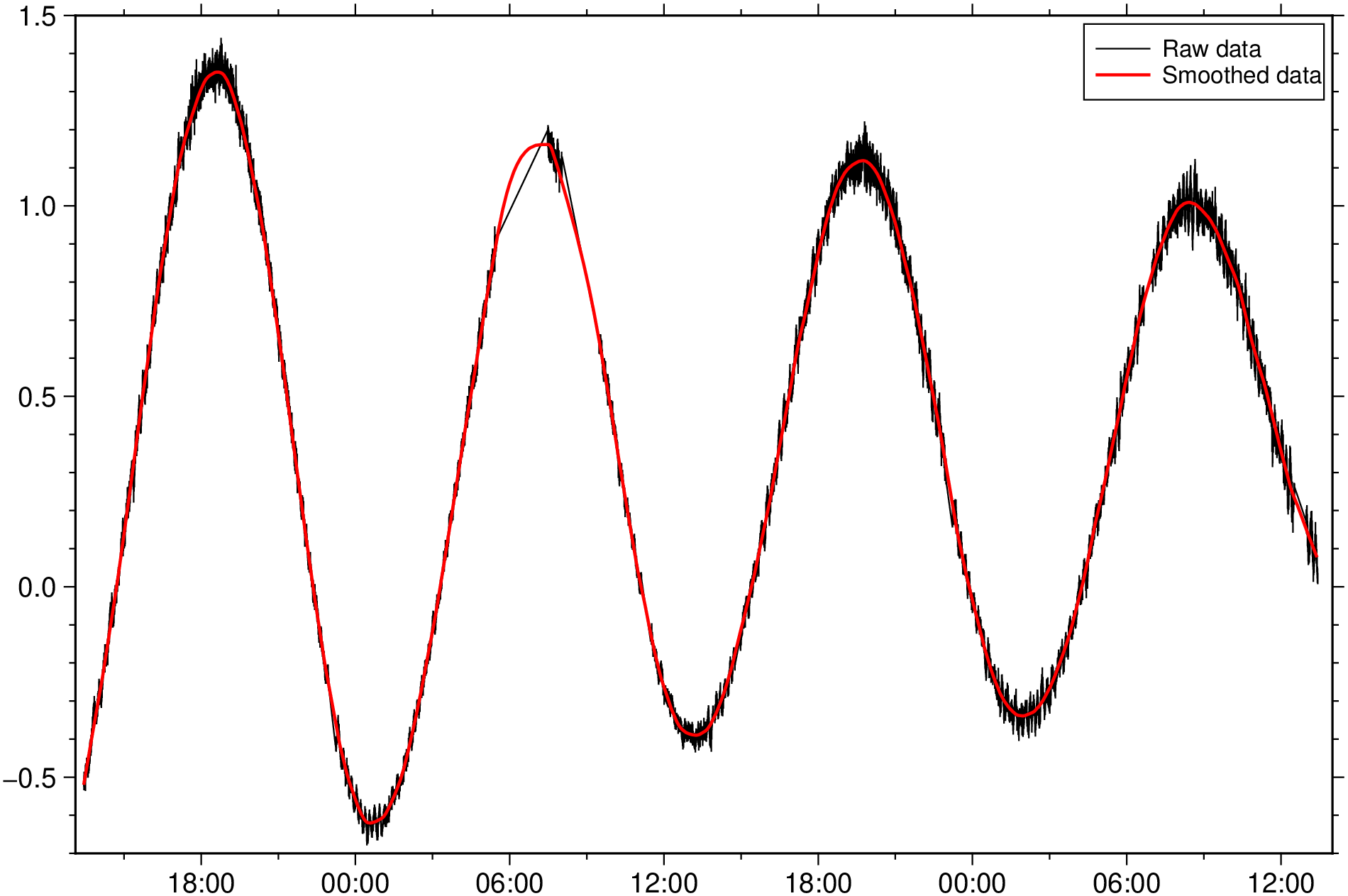
Dfinal = sample1d(Dl, T="2025-03-05T13:26:00/2025-03-07T13:24:05/60s");

And now we have a nice curve that we could use to calculate the derivatives or feed to an FFT to get the frequency components of the signal.

Show both original and smoothed data as points. It is not perfect at the top of the second creast but this was a tough case.

plot(D, legend= "Raw data")
plot!(Dfinal, lc=:red, lt=1, legend="Smoothed data", show=true)